Train Resistance
Aim - This page is dedicated to describing the different types of resistance that impact a trains and how they have been modelled within Open Rails.
If you wish to provide any feedback on this page, please use the contact page. It would be great to have some feedback, as this helps to ensure the accuracy of the information and model.
For information on how to apply resistance settings within Open Rails, refer to the Resistance Setting page.
Index
Resistance on straight and level track
Principles for Train Movement
Key Points to Remember
- Locomotive tractive effort must be greater then the train resistance forces.
- Train resistance is impacted by the train itself, curves, gradients, tunnels, etc.
- Tractive effort (force) reduces with speed, and will reach a point where it "equals" the train resistance, and thus the train will not be able to go any faster. This point will vary as the train resistance varies due to changing track conditions.
- For steam locomotive, the theoretical tractive effort is determined by the boiler pressure, cylinder size, drive wheel diameters, and will vary between locomotives. For diesels it is the power of the diesel prime mover(s) and the losses in the various conversion processes.
- Low Factors of Adhesion will cause the locomotive to slip.
Whilst this page is specifically aimed at steam locomotives, a lot of the principles, and physics are similar for diesel and electric locomotives.
Forces Impacting Train Movement
The steam locomotive is a heat engine which converts heat energy generated through the burning of fuel, such as coal, into heat and ultimately steam. The steam is then used to do work by injecting the steam into the cylinders to drive the wheels around and move the locomotive forward. The diesel has similarities in the fact that it relies on the burning of fuel oil to to drive a diesel engine, which generally is used to drive a generator, traction motors and finally a gearbox.
To understand how a train will move forward, it is necessary to understand the principle mechanical forces acting on the train. The diagram below shows the two key forces impacting on the ability for a train to move.
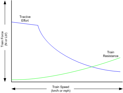
The driving force is the tractive effort ( Steam or Diesel ) produced by the locomotive, whilst the resisting force is the resistance presented by the train. Whilever the tractive effort is greater than the train resistance the train will continue to move forward, once the resistance exceeds the tractive effort, then the train will start to slow down, and eventually stop moving forward. The point where the two curves cross will be the "Balancing Speed", ie the maximum speed that the train can reach under the operating conditions described by the two force curves.
It should also be remembered that the "Adhesive" force of the locomotive will also play a part in determining whether a train can exert its full tractive force or not. See the description of Adhesion to understand how this impacts the adhesive effort of the train.
The sections below describe in more detail the forces associated with train resistance.
Train Resistance
The movement of the train is opposed by a number of different forces which are collectively grouped together to form the "train resistance".
The main resistive forces are as follows:
i) Resistance on straight and level track - this is the basic resistance of a train when it is travelling on straight and level track.
ii) Gradient resistance - trains travelling up hills will experience greater resistive forces then those operating on level track.
iii) Curve resistance - applies when the train is traveling around a curve, and will be impacted by the curve radius, speed, and fixed wheel base of the rolling stock.
iv) Tunnel resistance - applies when a train is travelling through a tunnel.
In other words the the principal forces opposing the movement of the train will include:
Where:
i) Fl = Resistance (or Friction) on straight and level track
ii) Fg = Gradient resistance - trains travelling up hills will experience greater resistive forces then those operating on level track.
i11) Fc = Curve resistance - applies when the train is traveling around a curve, and will be impacted by the curve radius, speed, and fixed wheel base of the rolling stock.
iv) Ft = Tunnel resistance - applies when a train is travelling through a tunnel.
As noted in the Train Movement section, and highlighted in the first diagram in that section, the tractive effort must exceed the resistance force of the train to ensure that the train moves. The point where the tractive effort crosses the train resistance force curve will typically indicate the maximum speed that the train can travel under the prevailing conditions, such as gradient, curve radius, etc, that the train is currently experiencing.
Typically resistance force is expressed in lbf (Imperial) or N(ewtons) (metric). Resistance force is often also called "friction".
This page describes these different types of resistance values, as well as describing a track geometry designed to minimise the impacts and effects of the above resistances on the trains performance.
Resistance on straight and level track
The following information is summarised from various sourcesd including the Proceedings of the American Railway Engineering Association.
On straight and level track, the forces that oppose the movement of the train are:
i) Bearing resistance - the type of bearing used on the stock represents some of the force. Older style stock is typically fitted with journal type bearings, whereas newer stock is fitted with roller bearings, which come in standard models or low friction models. The journal type of bearings tended to be cheaper, but presented a higher value of resistance to train movement.
ii) Train dynamic friction losses - These include flange effects which are associated With lateral motion and the resulting friction and impact of the wheel flanges against the gage side of the rail. They vary with speed, rail alignment, track quality, the surface condition of the rail under load, the horizontal contour of the railhead, contour and condition of the wheel tread, and the tracking effect of the trucks. Also there are miscellaneous losses due to sway, concussion, buffing and slack-action.
iii) Atmospheric resistance - resistance due to both still air and wind. Typically this resistance was influenced by the cross sectional area of the train and its speed. At high speeds air resistance became especially important as it was based upon the square of the speed.
iv) Flange resistance - Rolling friction between wheel and rail. This can be considered a constant for a given quality of track.
Various tests made over the years have shown that the resistance to train movement can be determined using an empirical expression of the following form:
where:
Resistance = train resistance in lbf (often expressed in lbs per ton)
A = rolling resistance component independent of train speed, this term can also contain an allowance for "internal" mechanical friction due to the valve gear on a steam locomotive, or the transmission losses on a diesel or electric locomotive.
B = coefficient used to define train resistance dependent on train speed
C = streamlining coefficient used to define train resistance dependent on the square of the train speed, can include information about the frontal surface area of the wagon, and an allowance for the drag created by the wagon.
D = aerodynamic coefficient or polynomial function used to further define train resistance, often combined with C.
V = train speed in mph (or m/s depending upon the units of the A, B & C values)
As a broad correlation, the formula parameters equate to the different types of friction as described in the following table:
A |
B |
C & D |
|---|---|---|
Journal / Roller Bearing Resistance |
Flange friction |
Head-end wind pressure |
Rolling resistance |
Flange impact |
Skin friction on the side of the train |
Track resistance |
Rolling resistance wheel/rail |
Rear drag |
|
Wave action of the rail |
Turbulence between cars |
|
|
Yaw angle of wind tunnels |
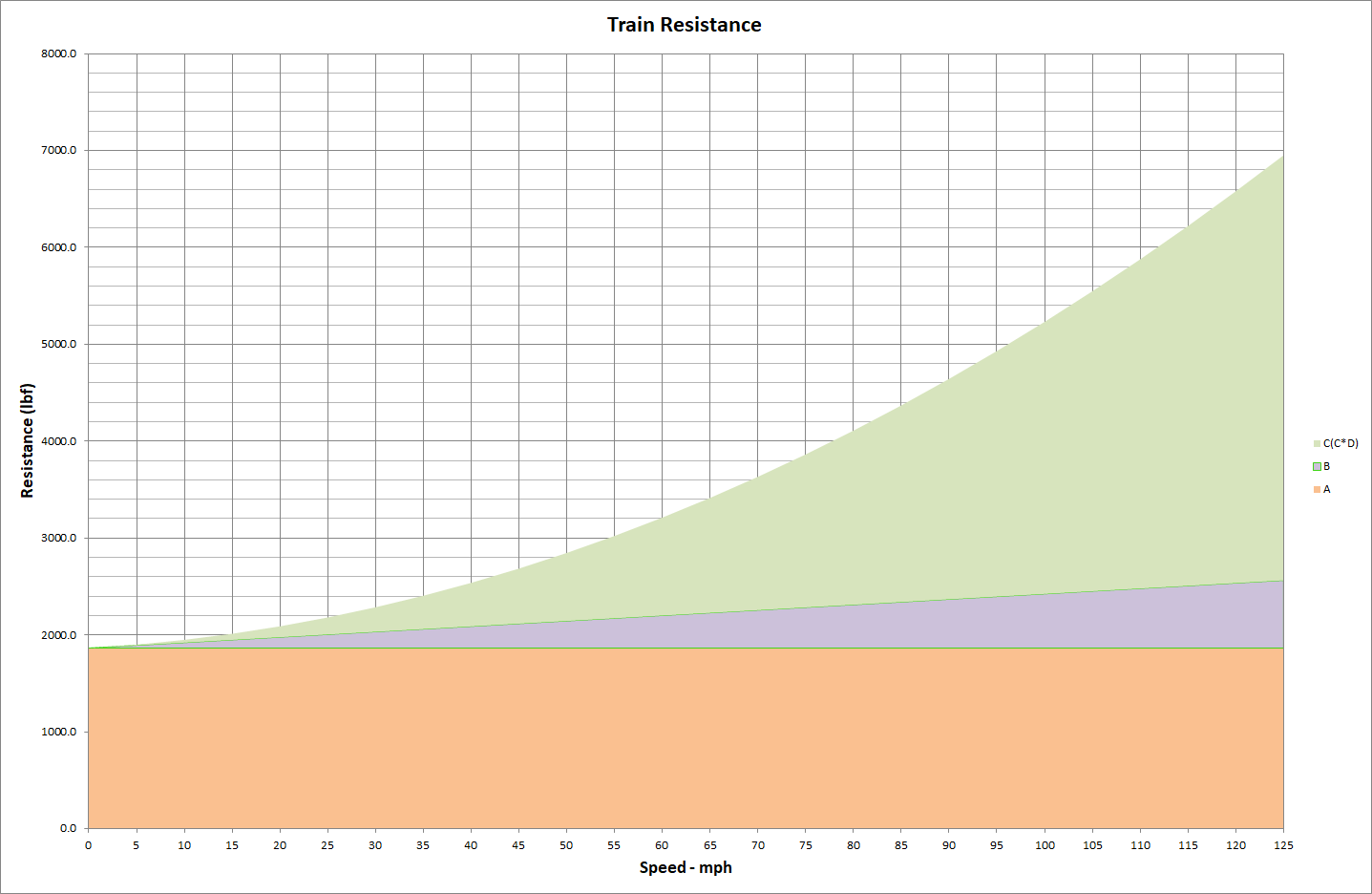
The impact of the respective coefficients on resistance is shown in the graph below.
From the graph it can be seen that the A value and the frictional elements that contribute to it (see table above) remain static regardless of the speed of the train. The B value can be seen to slowly increase with speed, whilst C & D values increase at a significant rate as the speed increases. This predominately represents the wind resistance of the stock. This also explains why so much attention is paid to high speed trains, and the need to streamline them.
Development of "Davis" Formula
Train resistance formulas were developed empirically by running a series of test on various train consists, and then fitting a quadratic formula to the test results.
American engineers did quite extensive testing and development of formulas. Professor Edward C. Schmidt was the first of a series of engineers who developed a set of formulas that were accepted by the railway community for use in calculating train resistance. His formulas were for freight wagons operating at speeds of up to 40mph by running a series of tests in 1910. In these days this speed range was considered satisfactory as the speed of freight trains rarely exceeded 40mph. In 1937, Professor J. K. Tuthill repeated the tests of Schmidt, and extended the tests up to speeds of 70mph.
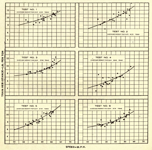
Schmidt and Harold Dunn ran a series of tests on Passenger Train Resistance. As part of this work the test results were plotted onto a graph, and a line of "best fit" was determined as shown on the following diagram. Typically the resistance of the complete train was measured, and then the weight of the train was used to calculate a resistance figure per ton. Over the years many researchers and railway companies have followed a similar approach to estimate the resistance of a train. These formula were valid up to 70mph.
Original Davis Formula
In 1926, W. J. Davis proposed an empirical formula for computing "Tractive Resistance of Electric Locomotives and Cars" moving on straight and level track. His formulas were primarily based upon the formulas of Schmidt (as Tuthill hadn't undertaken his tests until 1937), and his proposed values for the coefficients A, B and C & D shown above were as follows: This formula took the form shown below, and was correlated to various parameters of the train, such as the weight of the wagon, number of axles, and cross sectional area.
The original formula proposed by Davis (for freight cars) for cars with axle weights in excess of 5 tons (us) was as follows:
For lighter vehicles, ie axle weight less then 5 tons (us):
where:
w = Weight per axle (tons US)
V = train speed (mph)
a = Car cross sectional area (square feet)
n = Number of axles per car
NB: Weight is in US tons (2000lbs)
The original Davis formula has given satisfactory results for older equipment with journal (or friction) bearings within a speed range between 5 and 40 mph. Over the years the formula have been adjusted for higher speeds, roller bearings, increased dimensions and heavier loading of freight cars and changes in the track structure have made it desirable to modify the constants in the Davis equation.
The above formula is for a standard freight car, and can be adjusted by replacing the B, D and a values with those recommended by Davis from the following table as appropriate, and using the approximate cross section areas provided.Wagon Type |
a (sq ft) |
B |
D |
|---|---|---|---|
Locomotive - 50 tons |
105 |
0.03 |
0.0024 (0.0017 - Streamlined - Parabolic) |
Locomotive - 70 tons |
110 |
0.03 |
0.0024 (0.0017 - Streamlined - Parabolic) |
Locomotive - > 100 tons |
120 |
0.03 |
0.0024 (0.0017 - Streamlined - Parabolic) |
Freight Cars |
85-90 |
0.045 |
0.0005 |
Passenger Car (Vestibule ends) |
120 |
0.03 |
0.00034 |
Passenger Car (Open ends) |
120 |
0.03 |
0.0005 |
Multiple Unit Trains - leading (car vestibuled) |
80-110 |
0.045 |
0.0024 |
Multiple Unit Trains - trailing cars |
80-110 |
0.045 |
0.00034 |
Motor Cars - single |
80-95 |
0.09 |
0.0024 |
2 Axled Wagon (Safety Car Type) |
70-75 |
0.09 |
0.0024 |
Explanatory Notes -
- The first two terms of the equations represent journal friction almost entirely. They have been derived from dynamometer and coasting tests on standard freight and passenger cars and electric locomotives and are based on oil lubrication with average temperature conditions. Journal friction may be increased 20 to 40 per cent at temperatures below freezing.
- The third term comprises resistances due to flange friction, concussion, swaying, and miscellaneous frictions proportional to the speed. The factor for this element is decreased by increases in length of truck wheel base and increased by poor road bed conditions and inferior riding qualities of motor cars.
- The last term gives air resistance for average weight of car or locomotive in pounds per ton for standard types of equipment. No allowance is made for head winds or strong side winds.
- Locomotive resistance represents tractive effort delivered to driving axles and does not include friction losses in gears, motor bearings or other parts of the driving equipment, as there are usually covered in the motive power efficiency.
- The formulas are based on tests taken under mild weather conditions. Values obtained from them may be used as found in calculations relating to electric distributing systems, substations, energy consumption, and power demand. In the determination of electric motor characteristics and gear reductions to meet particular speed requirements, however, it may be desirable to add a small percentage to the required speed as a protection against unusual conditions.
- Locomotive resistance represents tractive effort delivered to driving axles and does not include friction losses in gears, motor bearings or other parts of the driving equipment, as these are usually covered in the motive power efficiency, and also applies to the driver tractive effort of steam locomotives. The mechanical resistance of steam locomotives equals 20 lb. per ton weight on drivers, hence should be added to locomotive resistance when applied to cylinder or indicated tractive effort. [This last note was added as a recommendation by AREA in 1943, and required the addition of 20 x Weight on Drivers to the Davis formula].
Trailing locomotive can use a B value similar to either one of the passenger cars depending upon their aeronomical design.
2 axle wagons, such as British Rail stock, etc, uses the following variations, A = low weight option, B = 0.09, and C = 0.0005 or 0.00034, depending upon whether it is an open or covered van type wagon.
Modified Davis Formula (1970)
The original Davis formula gave satisfactory results for older freight equipment with journal bearings within a speed range between 5 and 40 mph. However, roller bearings, increased dimensions and heavier loading of freight cars, the much higher operating speeds of freight trains, and changes in the track structure made it desirable to modify the constants in the Davis equation. Based upon work done by Committee 16 of the AREA, in 1970, the following modified formula was developed to allow for improvements in technologies, and operating practices.
Where the parameters are the same as above with the following parameter added:
K = air resistance (drag) coefficient. Typical values are 0.076 for conventional equipment, 0.0935 for containers, and 0.16 for trailers on flat cars.
Other types of car not specified above will have use the original Davis formula, alternatively perhaps a combination of the A and B values from this formula, and the C value from the original Davis formula.
Davis Formula (1992 Canadian National variation)
The original train resistance formula has been retained as to form, but over the years different coefficients have been developed to reflect changes such as higher speeds, more modem equipment, and today's track and truck designs.
The 1992 Canadian National version of the train resistance formula is presented below. When used with the coefficients shown (many of which have been developed in dynamometer car tests), the formula has given reliable results in train performance calculator programs or similar applications.
where:
W = Total Weight (tons US)
V = train speed (mph)
a = Car cross sectional area (square feet)
n = Number of axles per car
C = Canadian National streamlining coefficient
The following table shows the range of values for the C coefficient for various kinds of equipment. Note that these values for C are scaled for use with the Canadian National formula only.
Degree of Streamlining |
Example Equipment |
C (Cn Coefficient) |
|
|---|---|---|---|
Leading Eqpt. |
Trailing Eqpt. |
||
Nil 1 |
Open auto transporter |
- |
12.3 |
Nil 2 |
Freight locomotive |
24.0 |
5.5 |
- |
Mixed consist of freight cars |
- |
5.0 |
Low 3 |
RDC |
19.0 |
3.5 |
Low 4 |
Conventional passenger incl. loco. |
19.0 |
3.5 |
Med 5 |
- |
14.0 |
3.0 |
Med 6 |
- |
10.0 |
2.6 |
High 7 |
High Speed Passenger |
7.6 |
2.3 |
High 8 |
Maximum possible streamlining |
7.0 |
2.0 |
When certain types of cars predominate in a train more accurate resistance values for such a train can be obtained by using C coefficients from the following table. The table shows in more detail recommended Canadian National values for C and cross-sectional areas for the various equipment types.
Type of Equipment |
Cn Coefficient |
Coefficient Area (sq ft) |
|---|---|---|
Box Car |
4.9 |
140 |
Bulkhead Flat (loaded) |
5.3 |
140 |
Bulkhead Flat (empty) |
12.0 |
140 |
Coal Gondola (loaded) |
4.2 |
105 |
Coal Gondola (empty) |
12.0 |
105 |
Covered Hopper |
7.1 |
125 |
Tank Car |
5.5 |
95 |
Standard Flat Car (without trailers) |
5.0 |
25 |
Standard Flat Car (with trailers) |
5.0 |
125 |
Caboose |
5.5 |
145 |
Conventional Passenger Coach |
3.5 |
130 |
Modern Lightweight Passenger Equipment |
2.0 |
110 |
Leading Freight Locomotive |
24.0 |
160 |
Multi-level Auto Transporter (open) |
12.3 |
150 |
Multi-level Auto Transporter (closed) |
7.1 |
170 |
Air Drag
The above Davis formula have been develop without any allowance for the impact of wind, see later description, however a train will suffer from a certain amount of air drag as the train moves still air. As air drag impacts the C value in the formula it will increase dramatically as the speed increases (due to V^2 multiplication). For low speed freight trains this was not considered a big issue, but as passenger train speeds were increased more attention was paid to the impact of drag.
To reduce drag some degree of streamlining was introduced to the train. The streamlining could either be added to the leading vehicle (typically the locomotive), the cars, or both. The diagram below shows some typical types of "noses" for locomotives, and the table underneath shows the type of drag reduction that might be expected (Information taken from The Steam Locomotive by Ralph P. Johnson).

Flat |
Parabolic |
Parabolic Wedge |
100% |
65% |
50% |
|---|
In his book "Tractive Resistance of Diesel Railcars and Locomotives", J. L. Koffman suggests, "Simple square (flat) ends with well-rounded corners, should be used with vehicles operating at a maximum speed of up to 50 m.p.h., and well-rounded ends (parabolic) should be used with vehicles not exceeding 80 m.p.h. Vehicles operatiog at up to 100 m.p.h should be provided with elliptic ends (parabolic wedge)."
Koffman goes onto suggest that adding different skirt combinations can achieve some additional improvement in air drag as well. The diagram below shows the suggested reductions with different skirt combinations.
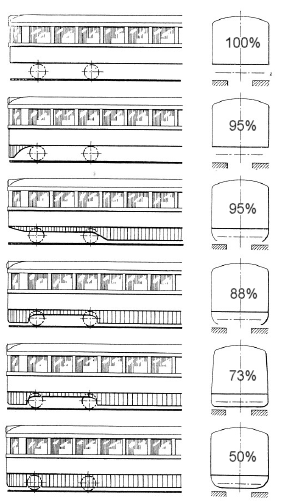
Naturally this is a very complex subject, and the above information offers an approximate view of how air drag can be changed by design of the wagon.
Note: It should also be noted that formulas developed for a specific piece of rolling stock will most likely have these factors already built into them. Whereas generic formulas, such as the original Davis formulas, and the 1970 versions are developed with minimal air drag reduction. The 1992 version, based upon the Canadian Railways version, does include allowances for different types of drag. The earlier Davis formulas were developed for vestibule cars (ie enclosed ends), so it would be reasonable to expect that open ended cars would have a slightly higher value of drag (possibly 147%)
Comparison of Different Resistance Calculations
The following curves for different types of stock show the variety of resistance values that can be obtained. They also demonstrate the value of using known resistance curves when thay are available.
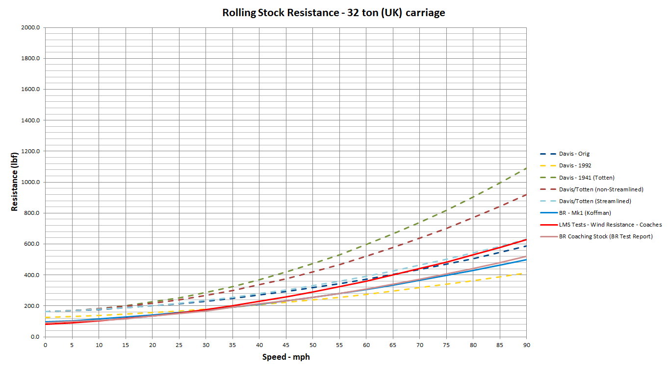
Passenger StockThe first curve represents Passenger Stock and shows the various Davis variations (shown with dotted curves) against three curves (shown in solid curves) provided by UK railway companies. The LMS curve were used for testing in the 1933, whereas the BR Coaching stock curve was measured during testing of the Duke of Gloucester locomotive, and the Mark1 (Mk1) passenger stock curve was taken from a report by Koffman, which were introduced from the early 1950s.. Some of the differences between these curves can possibly be attributed to the change in design of the vehicles between the 1930s and 1950s, as well as differences in streamlining, etc. Possible differences between the Davis curves and the curves taken from BR literature could be more to do with the A and B parameter, which impacts the curve more towards lower speeds. Thus there could be differences in the type of journal bearings used in these cars, as well as track designs and standards could be different between the UK and US.
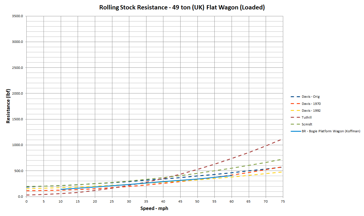
The BR flat wagon curve was taken from a 1964 publication by Koffman.
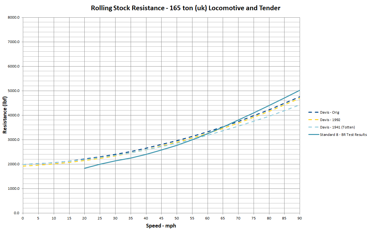
The graph for the locomotive shows the combined resistance of the locomotive and the tender. It shows the curve taken from a BR Test report for the Duke of Gloucester locomotive, and the curves predicted using the Davis variation formulas.
It should be noted that strictly speaking the 1992 variation of the Davis equation was probably not pertinent to the steam locomotive as most, if not all steam locomotives were no longer operated by the Canadian National Railway at the time the formula was adjusted. It would apply to diesel and electric locomotives.
The diagram shows the original Davis formula, as well as the modified and adjusted values, and also curves based upon Canadian National Railways and British Rail information. It can be seen that the curves diverge significantly at higher speeds. It should however be noted, that whilst the diagram speed axis has been extended to 125mph, it is unlikely that freight stock would reach this type of speed. Therefore a more realistic view can be obtained by comparing the curve differences around the 60mph point.
To demonstrate some different formulas that have been developed for specific stock over the years, Darwin Smith has produced a summary of different resistance formulas found by an Internet search. This summary and a spreadsheet enabling the user to undertake some calculations is available in a Friction Calculator (Updated Oct 2020) package.
For information on setting the Davis values in the WAG or ENG file, refer to Level Resistance setting and Resistance Calculation page.
Starting Resistance
To start a train the locomotive must produce enough tractive force to overcome the following two factors:
- Vehicle Internal Resistance - this is the resistance to movement by the wheel bearing. Depending upon the weight per axle, the bearing type and the temperature of the bearings, which is in turn a function of
both the ambient temperature and the length of time the equipment has been stopped, starting resistance for "solid" type bearings may be as high as 35 lbs per ton (US) below 30 degrees F. An average value for light and heavy cars of 25 lbs per ton (US) at starting is sometimes considered a "reasonable" value for above-freezing temperatures. The starting resistance of roller bearings is much lower, and a general resistance value of 5 lb/ton (US) (or less) might be considered a satisfactory estimate for roller-bearing equipment at above-freezing temperatures.
The vehicle internal resistance of the train will typically reduce as the wheel bearing heats up as the vehicle is in motion. - Track Resistance - can be caused by the flattening of the wheel tyre, and the rail at the point of contact. However modern steel wheels are considered hard enough to make this factor insignificant. Hence the principal track resistance comes about as a result of the depression or downward deflection of the track due to the weight of the wagon. The amount of depression will vary due to the axle weights on the track, and how rigid the design of the track is. The diagram below demonstrates an exagerated depression of the track (blue line) due to the weight of the wagon. As can be imagined, as the train starts, each wheel in the train must climb a small gradient. When the train starts moving and the speed of the train increases, the track tends to "flatten" out, and eventually only the leading wheels of the train depress the track.

Dendy Marshall in his work on train resistance published the following formulas to calculate the starting resistance.
He further defined
where:
K = resistance factor derived empirically from tests.
Wg = Gross Weight of the Vehicle (tons UK)
and
where:
Wa = Axle Weight (tons UK)
Ad = angle of depression
Typically most couplers allow some amount of slack between cars. Provided the train is "bunched" up with the couplers pushing against each other, this slack can be used to start the train one car at a time, which allows the starting resistance to reduce on the first car before the last car in the train starts to move. If the train is stretched with the maximum amount of slack already in the couplers, then the locomotive must then pull the train with the combined starting resistance of each car. Sometimes the driver may reverse the train slightly to "bunch" it up so that the benefit of coupler slack can be used. When attempting to start a train on a gradient, it may not be possible to "bunch" the train up, and so the the train will need to start with the full starting resistance. Railway companies usually take these types of conditions into account when they are setting load tonnage ratings.
Wheel Bearing Temperature
When first developed railways used 'plain bearings' (sometimes also called friction) on their wagons. Typically these types of bearings were compact, lightweight, and very economical. They suited the low speed of operations of the railways in this era.
As the speed of railways accelerated from the mid 20th Century, it was found that despite their cost roller bearings were more efficient, and suitable for railway operations. Hence most railways started to use roller bearings on their higher speed stock.
Both of the above bearing types generate friction as they rotate, and hence heat is generated. Depending upon many factors, including bearing type, housing design, lubricant used, etc, the heat generated will be matched by the heat dissapated from the bearing by the surrounding air, and hence an equilibrium temperature will be reached. Under normal operating conditions a railway wheel bearing should be within an approximate temperature range of 50-135 Deg C (120-275 DegF). Whilst the oil lubricant in a bearing is unlikely to freeze solid at temperatures below freezing point, it will loose some of it viscosity, and hence the bearing friction will increase significantly. This results in a higher level of resistance, as described in the section above.
If a bearing is damaged or poorly maintained then the bearing will need to overcome extra friction, and hence higher temperatures of operation will result. Wheel bearings operating at elevated temperatures are often called Hotboxes, and may result in damaged wheelsets, and in extreme circumstances fires, and derailments.
In earlier times railways had procedures whereby trains were inspected at selected intervals for hotboxes, and in more recent years, railways have deployed detectors to identify overheating bearings at selected points along their railway routes.
Wind Resistance
The Davis resistance formula described in the section above was developed for STILL conditions, ie with no wind movement. The third component (i.e. R3 = C * D * V2) of the Davis formula models the impact of drag as the train moves through still air. Drag is significantly impacted by the speed of the train, and hence drag becomes a big issue with high speed trains, whereas low speed trains are not as effect by drag issues.
The presence of a wind can, for high speed operations, significantly add to the resistance impacting upon the train. The following is a brief overview of one method to approximate this impact. To accurately assess the impact it is often necessary to undetake wind tunnel tests. Typically for modern high speed trains this is part of the design process.
The Davis models the impact of drag by the setting the third element of the equation to the following form:
Where:
R3 = Third Resistance element of wagon (lbf)
K = Factor allowing for impacts of wind, track condition, etc.
A = Frontal area of wagon (ft2)
V2 = speed of train (mph)
The total wind resistance impact upon train operation is calculated by the following formula:
Briefly these two components are described below
Wind Drag Resistance (Rdrag) - If a train is heading into a headwind then the train will experience greater resistance to movement, similarly if the train has a tailwind, then the trains resistance will decrease as the wind provides a "helping hand". As the wind swings from the head of the train to the rear resistance will decrease. When the wind is perpendicular to the train, drag impact due to the wind will be zero.
Lateral Force Resistance (Rlateral) - When the wind blows from the side of the train, the train will be pushed against the outside track rail, thus increasing the amount of resistance experienced by the train.
As suggested in the introduction, drag is heavily dependent upon the velocity of the train. When a wind is present, then the resultant velocity of the train and the wind is calculated, and inserted into the above equation.
The following diagram demonstrates a typical vector diagram for the train movement and wind.
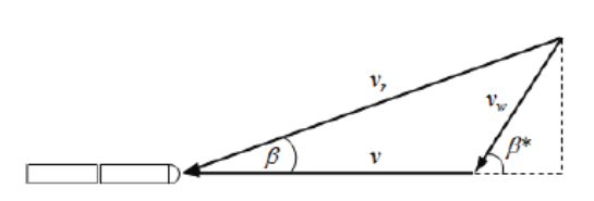
Where:
V = train speed and direction
Vw = wind speed and direction
Vr = resultant combined train and wind speed magnitude
B* = wind direction
B = resultant combined train wind direction
The 1942 AREA proceedings (pg 56) provide the following formula to calculate the lateral force resistance:
Where
Rlateral = unit locomotive side wind resistance-lb. per ton
f =coefficient of friction between wheel and rail
W = locomotive weight-tons (US)
C and K = constants dependent upon vehicle contour
B = angle between locomotive and wind directions - degrees
VL = locomotive speed - mph
a and c = constants calculated based upon train and wind speed.
For information on setting values for wind resistance in the WAG or ENG file, refer to wind Resistance setting page.
Gradient Resistance
The gradient resistance is the extra force required to lift a train up a gradient, or conversely is the extra force "pushing" the train down a hill.
It is a positive quantity when going up the grade and a negative quantity for going down the grade.
As shown in the diagram below the work of lifting a weight W up a distance represented by BC is equal to the work required to overcome the resistance R (due to grade only) through a distance AB, ie W x BC = R x AB.
Thus the following formula can be used to calculate grade resistance:
or alternatively
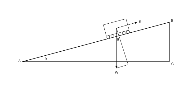
where:
Grade resistance = Grade resistance in lbf (often expressed in lbs per ton)
W = load in tons
TR = (vertical rise / length of incline)
This is calculated in Open Rails automatically.
Curve Resistance
When a train travels around a curve, due to the track resisting the direction of travel (ie the train wants to continue in a straight line), it experiences increased resistance as it is "pushed" around the curve.
Over the years there has been much discussion about how to accurately calculate curve friction. The calculation methodology presented (and used in OR) is meant to be representative of the impacts that curve friction will have on rolling stock performance.
Factors Impacting Curve Friction
A number of factors impact upon the value of resistance that the curve presents to the trains movement, and these are as follows:
i) Curve radius - the tighter the curve radius the higher the higher the resistance to the train
ii) Rolling Stock Rigid Wheelbase - the longer the rigid wheelbase of the vehicle, the higher the resistance to the train. Modern bogie stock tends to have shorter rigid wheelbase values and is not as bad as the older style 4 wheel wagons.
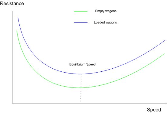
iii) Speed - the speed of the train around the curve will impact upon the value of resistance, typically above and below the equilibrium speed (ie when all the wheels of the rolling stock are perfectly aligned between the tracks). See the section below "Impact of superelevation".
The impact of wind resistance on the curve is ignored.
Impact of Rigid Wheelbase
The length of the rigid wheelbase of rolling stock will impact the value of curve resistance. Typically rolling stock with longer rigid wheelbases will experience a higher degree of "rubbing" or frictional resistance on tight curves, compared to stock with smaller wheelbases.
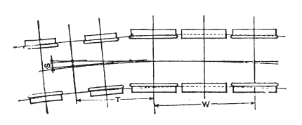
Steam locomotives usually created the biggest problem in regard to this as their drive wheels tended to be in a single rigid wheelbase as shown in the figure below. In some instances on routes with tighter curve the "inside" wheels of the locomotive was sometimes made flangeless to allow it to "float" across the track head. Articulated locomotives, such as Shays, tended to have their drive wheels grouped in bogies similar to diesel locomotives and hence were favoured for routes with tight curves.
The value used for the rigid wheelbase is shown as W in the diagram below.
Impact of SuperElevation
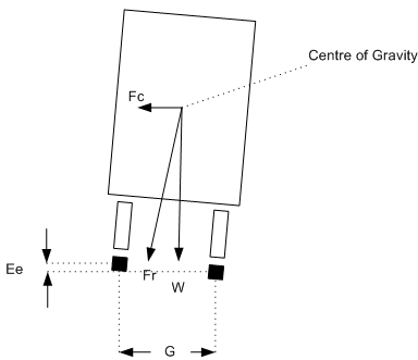
On any curve whose outer rail is super-elevated there is, for any car, one speed of operation at which the car trucks have no more tendency to run toward either rail than they have on straight track, where both rail-heads are at the same level (known as the equilibrium speed). At lower speeds the trucks tend constantly to run down against the inside rail of the curve, and thereby increase the flange friction; whilst at higher speeds they run toward the outer rail, with the same effect. This may be made clearer by reference to the figure below, which represents the forces which operate on a car at its centre of gravity. With the car at rest on the curve there is a component of the weight W which tends to move the car down toward the inner rail. When the car moves along the track centrifugal force Fc comes into play and the car action is controlled by the force Fr which is the resultant of W and Fc. The force Fr likewise has a component which, still tends to move the car toward the inner rail. This tendency persists until, with increasing speed, the value of Fc becomes great enough to cause the line of operation of Fr to coincide with the centre line of the track perpendicular to the plane of the rails. At this equilibrium speed there is no longer any tendency of the trucks to run toward either rail. If the speed be still further increased, the component of Fr rises again, but now on the opposite side of the centre line of the track and is of opposite sense, causing the trucks to tend to move toward the outer instead of the inner rail, and thereby reviving the extra flange friction. It should be emphasised that the flange friction arising from the play of the forces here under discussion is distinct from and in excess of the flange friction which arises from the action of the flanges in forcing the truck to follow the track curvature. This excess being a variable element of curve resistance, we may expect to find that curve resistance reaches a minimum value when this excess reduces to zero, that is, when the car speed reaches the critical value referred to. This critical speed depends only on the super-elevation, the track gauge, and the radius of track curvature. The resulting variation of curve resistance with speed is indicated in the diagram below.
Calculation of Curve Resistance
where:
R = Curve resistance
W = vehicle weight
F = Coefficient of Friction,
u = 0.5 for dry, smooth steel-to-steel, wet rail 0.1 - 0.3
D = track gauge
L = Rigid wheelbase
r = curve radius
Source: The Modern locomotive by C. Edgar Allen - 1912
Curve Speed
As has been described in the proceeding section, the permissible speeds that a train can travel around a curve becomes critical, and the three key speed limits are as follows:
- Equilibrium Speed - maximum speed around a curve which ensures that the load of the wagon is balanced across all the wheels, and that the forces between the wheels and track are equal. Speeds in excess of this value may result in uneven track wear and tear. This speed limit is mainly influenced by track superelevation.
- Unbalanced Speed - maximum speed around a curve which allows a certain amount of load unbalance between the wheels and the track. Typically the amount of unbalance is determined by the of the amount of unbalanced superelevation (cant deficiency) which is allowable by individual railway companies. The higher this value the greater the impact felt by passengers, and their level of discomfort in rounding the curve.
- Critical Speed - the speed at which the rolling stock is likely to overturn. Mostly impacted by the Centre of Gravity.
A formula in imperial units to calculate the Equilibrium Speed and Unbalanced Speed is:
V = speed ft/s
S = Superelevation in inches (includes both Balanced and Unbalanced values of superelevation, for Equilibrium speed only use the track superelevation, for Unbalanced speed sum the Balanced and Unbalanced superelevation values.)
g = Acceleration due to gravity (32.2 ft/s2)
r = Radius of curve in feet
G = Track gauge (note the distance between rail centres, and not the inside rail measurement)
To calculate the Critical Speed, the Centrifugal Force (Fc above) balances the overturning weight (W above)of the wagon:
V = speed ft/s
F = Centrifugal force in tons (acting on the point of centre of gravity)
g = Acceleration due to gravity (32.2 ft/s2)
r = Radius of curve in feet
W = Weight of the Vehicle in tons
To gain a sense of how the speed around a curve will vary under different conditions, refer to the calculators shown on the Curve Speed Test page. Also refer to this page when testing rolling stock to see how it will perform for different curve scenarios.
Calculation of Speed Impact on Curve Resistance
As described above the least value of resistance will occur at the equilibrium speed, and as the speed increases or decreases from the equilibrium speed, the value of curve resistance will increase accordingly. This concept is shown pictorialy in the following graph.
Open Rails uses the following formula to model the impact of speed upon the curve resistance:
Typical Rigid Wheelbase Values
The following values can be used as defaults where actual values are not readily available from rolling stock plans.
Rolling Stock Type |
Typical value |
|---|---|
Freight Bogie type stock (2 wheel bogie) |
5' 6" (1.6764m} |
Passenger Bogie type stock (2 wheel bogie) |
8' (2.4384m) |
Passenger Bogie type stock (3 wheel bogie) |
12' (3.6576m) |
Typical 4 wheel rigid wagon |
11' 6" (3.5052m) |
Typical 6 wheel rigid wagon |
12' (3.6576m) |
Tender (6 wheel) |
14' 3" (4.3434m) |
Diesel, Electric locomotives |
Similar to passenger stock |
Steam locomotives |
Dependent on# of drive wheels, Can be up to 20'+ , eg large 2-10-0 locos |
Modern publications suggest that an allowance of approximately 0.8 lb. per ton (us) per degree of curvature for standard gauge tracks. At very slow speeds, say 1 or 2 mph, the curve resistance is closer to 1.0 lb. (or 0.05% up grade) per ton per degree of curve.
For information on setting the curve resistance in the WAG or ENG file, refer to Curve Resistance setting page.
Tunnel Resistance
Introduction
When a train travels through a tunnel it experiences increased resistance to the forward movement.
Over the years there has been much discussion about how to accurately calculate tunnel resistance. The calculation methodology presented (and used in OR) is meant to provide a indicative representation of the impacts that tunnel resistance will have on rolling stock performance.
Factors Impacting Tunnel Friction
In general, the train aerodynamics are related to aerodynamic drag, pressure variations inside train, train-induced flows, cross-wind effects, ground effects, pressure waves inside tunnel, impulse waves at the exit of tunnel, noise and vibration, etc. The aerodynamic drag is dependent on the cross-sectional area of train body, train length, shape of train fore- and after-bodies, surface roughness of train body, and geographical conditions around the traveling train. The train-induced flows can influence passengers on a subway platform and is also associated with the cross-sectional area of train body, train length, shape of train fore- and after-bodies, surface roughness of train body, etc.
A high speed train entering a tunnel generates a compression wave at the entry portal that moves at the speed of sound in front of the train. The friction of the displaced air with the tunnel wall produces a pressure gradient and, as a consequence, a rise in pressure in front of the train. On reaching the exit portal of the tunnel, the compression wave is reflected back as an expansion wave but part of it exits the tunnel and radiates outside as a micro-pressure wave. This wave could cause a sonic boom that may lead to structural vibration and noise pollution in the surrounding environment. The entry of the tail of the train into the tunnel produces an expansion wave that moves through the annulus between the train and the tunnel. When the expansion pressure wave reaches the entry portal, it is reflected towards the interior of the tunnel as a compression wave. These compression and expansion waves propagate backwards and forwards along the tunnel and experience further reflections when meeting with the nose and tail of the train or reaching the entry and exit portals of the tunnel until they eventually dissipate completely.
The presence of this system of pressure waves in a tunnel affects the design and operation of trains, and they are a source of energy losses, noise, vibrations and aural discomfort for passengers. These problems are even worse when two or more trains are in a tunnel at the same time. Aural comfort is one of the major factors determining the area of new tunnels or the maximum train speed in existing ones.
Importance of Tunnel Profile
As described above, a train travelling through a tunnel will create a bow wave of air movement in front of it, which is similar to a "piston" effect. The magnitude and impact of this effect will principally be determined by the tunnel profile, train profile and speed.
Typical tunnel profiles are shown in the diagrams below.

As can be seen from these diagrams the smaller the tunnel cross sectional area compared to the train cross sectional area, the less air that can "escape" around the train, and hence the greater the resistance experienced by the train. Thus it can be understood that a single train in a double track tunnel will experience less resistance then a single train in a single track tunnel.
Source: Reasonable compensation coefficient of maximum gradient in long railway tunnels by Sirong YI, Liangtao NIE, Yanheng CHEN, Fangfang QIN
For information on setting the curve resistance in the WAG or ENG file, refer to Tunnel Resistance setting page.
Track Geometry
Most railway companies have established track geomety standards to ensure that the construction and maintenance of tracks is undertaken within safe limits, prevent excessive forces on rolling stock and tracks to minimise wear and tear, ensure passenger comfort and finally to ensure that trains are able to perform at their optimal level of efficiency. The track geometry has typically been improved over the years as the need for higher speed, heavier loads, and passenger comfort have been identified. The table and notes below summarises the principle track geometry parameters currently used for New South Wales mainline routes. Branchlines and older routes may be built or operate on more onerous standards. Additional parameters and a more detail explanation can be found in ESC 210 - Track Geometry and Stability.
For the sake of comparison with older standards, imperial figures have been included in barackets after each of the parameters below, and they have been rounded to the relevant imperial value.
| Parameter | Mixed Passenger / Freight Main Line |
Maximum (or Minimum) Limits | ||
|---|---|---|---|---|
| Track Gauge | 1435mm (4ft 8.5in) | 1435mm (4ft 8.5in) | ||
| Speed | Normal | 115km/h (70mph) | 115km/h (70mph) | |
| XPT | 160km/h (100mph) | 160km/h (100mph) | ||
| Minimum Curve Radius | 400m (20chs or 1312ft) | 160m (8chs or 525ft) | ||
| Superelevation (or Cant) | Mainline | 125mm (5.0in) | 140mm (5.5in) | |
| Platform (New) | 60-100mm (2.5-4.0in) | 75-100mm (3.0-4.0in) | ||
| Turnout | 50mm (2.0in) | 50mm (2.0in) | ||
| Superelevation (or Cant) Deficiency(+)/Excess(-) | Plain Track | Normal | +/-75mm (3.0in) | +80/-75mm (+3.1/-3.0in) |
| XPT (T1) | +110/-75mm (+4.25/-3.0in) | +110/-75mm (+4.25/-3.0in) | ||
| Turnout Track (Conventional) | Normal | 75mm (3.0in) | 140mm (5.5in) | |
| XPT (T1) | 75mm (3.0in) | 140mm (5.5in) | ||
| Diamond Crossing | Normal | 0mm (0.0in) | 25mm (1.0in) | |
| XPT (T1) | 0mm (0.0in) | 25mm (1.0in) | ||
| Gradient (compensated) | Mainline | 1 in 100 (1.0%) | Ruling Gradient | |
| Platform | 1 in 150 (0.67%) | 1 in 100 (1.0%) | ||
Cant Deficiency - the train is allowed to exceed the Equilibrium Speed by an amount determined by the Cant Deficiency. In this scenario the outer wheels on the bogie have more apparent weight upon them.
Cant Excess - determines the minimum ideal speed around the curve, i.e. the speed less then the Equilibrium Speed. In this instance the Cant is deemed to be in Excess. In this scenario the inner wheels on the bogie have more apparent weight upon them.
Ruling Gradient - is typically the steepest gradient on a section of line in a particular route or section thereof. Normally train loads were calculated so that a single steam locomotive could successfully haul the load up the gradient. Sometimes, where it was operationally expedient and efficient to do so a bank (or helper) locomotive was employed to assist the train locomotive in hauling the train to the top of the grade.
Gradient (Compensated) - As suggested in the section above on curve resistance, when traveling around a curve a train will encounter greater resistance then on a straight and level track. Railways often equate this to an amount of gradient that a train will face, thus if a train is traveling up a grade and encounters a sharpe curve then the equivalent gradient that the train is facing will be greater then that experienced on the level graded track. On modern designed tracks the gradient on a curve can be eased by a relevant amount to ensure that the ruling gradient on the slope is consistent throughout the climb. On older lines, where the curves were often laid on the same gradient as the straight track, the ruling gradient for section will be increased by the amount of impacted of the sharpest curve on the section.
The compensated gradient can be found from the formula:
Thus for example, if a 1 in 100 (1.0%) gradient has a 300m curve located on it, then a grade compensation of 0.2% must be applied. Hence to maintain the 1 in 100 ruling grade, the curve can be laid on a 1 in 125 (0.8%) grade, or alternatively if the curve is laid on a 1 in 100 grade then the ruling gradient must be changed to 1 in 83 (1.2%). Train loads will need to be calculated accordingly.